Terrain, land cover, population and protected areas
Source:vignettes/articles/terrain-population.Rmd
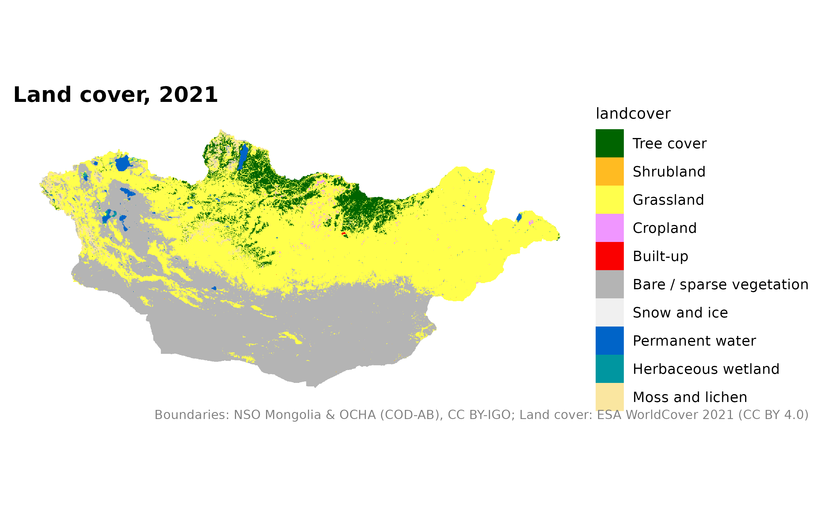
terrain-population.RmdThese layers are rasters (grids of cells), returned as
terra SpatRasters. National 1 km grids are downloaded once
and cached; finer grids are read directly from the cloud for one area at
a time.
| Function | Resolutions | Source |
|---|---|---|
mn_elevation(), mn_hillshade()
|
1 km (national), 90 m (by area) | Copernicus DEM GLO-90 |
mn_landcover() |
1 km (national), 10 m (by area) | ESA WorldCover 2021 |
mn_population() |
1 km, 100 m; years 2015 to 2030 | WorldPop |
mn_map() draws rasters too, with the right colours and
credits.
Terrain
mn_map(mn_elevation(), title = "Elevation (m)") +
  geom_sf(data = mn_aimags(), fill = NA, colour = "white", linewidth = 0.2)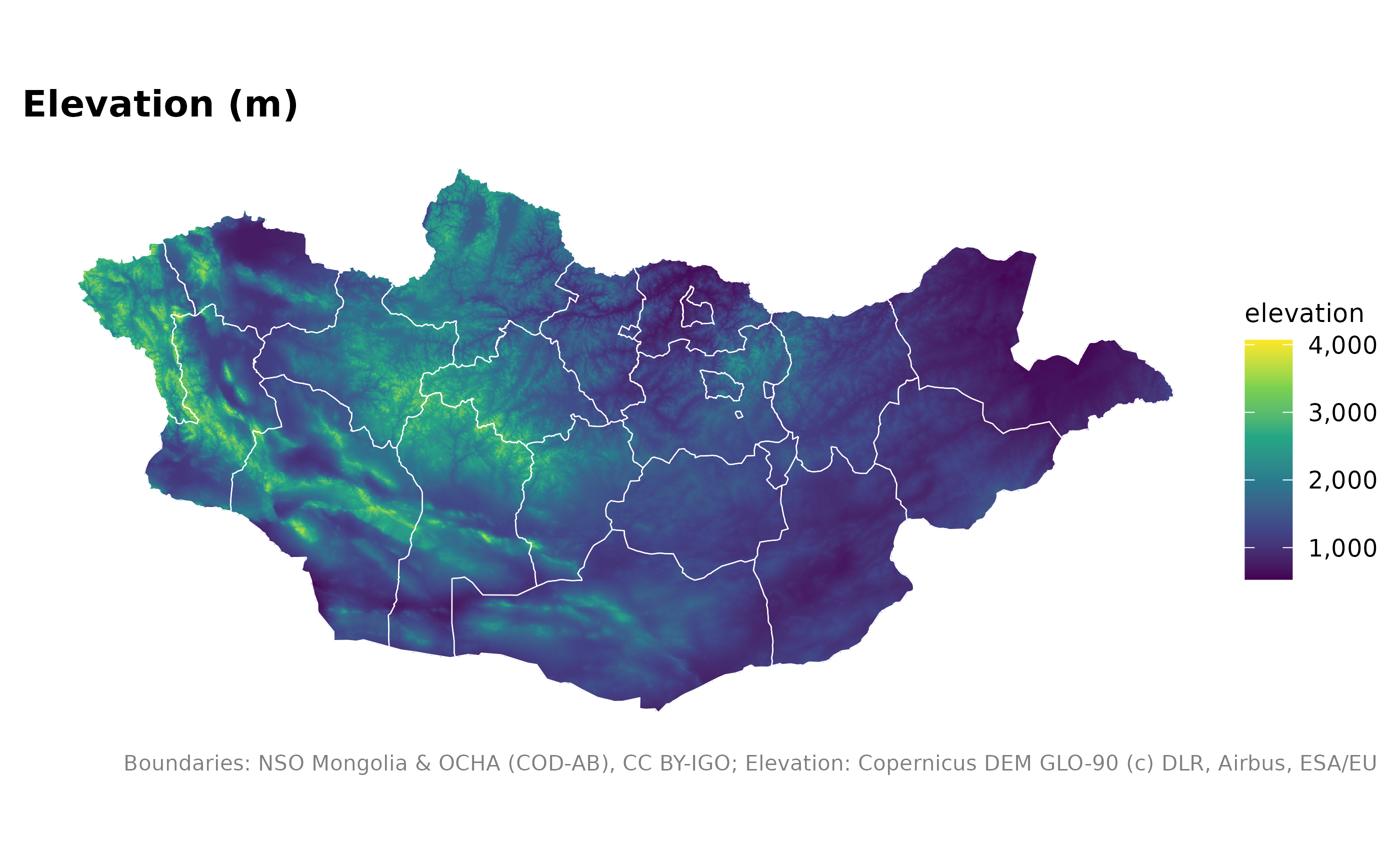
Shaded relief makes a good background under other layers:
mn_map(mn_hillshade(), caption = FALSE) +
  geom_sf(data = mn_aimags(), fill = NA, colour = "white", linewidth = 0.3) +
  geom_sf(data = mn_settlements(type = c("capital", "aimag_centre")), colour = "firebrick", size = 1)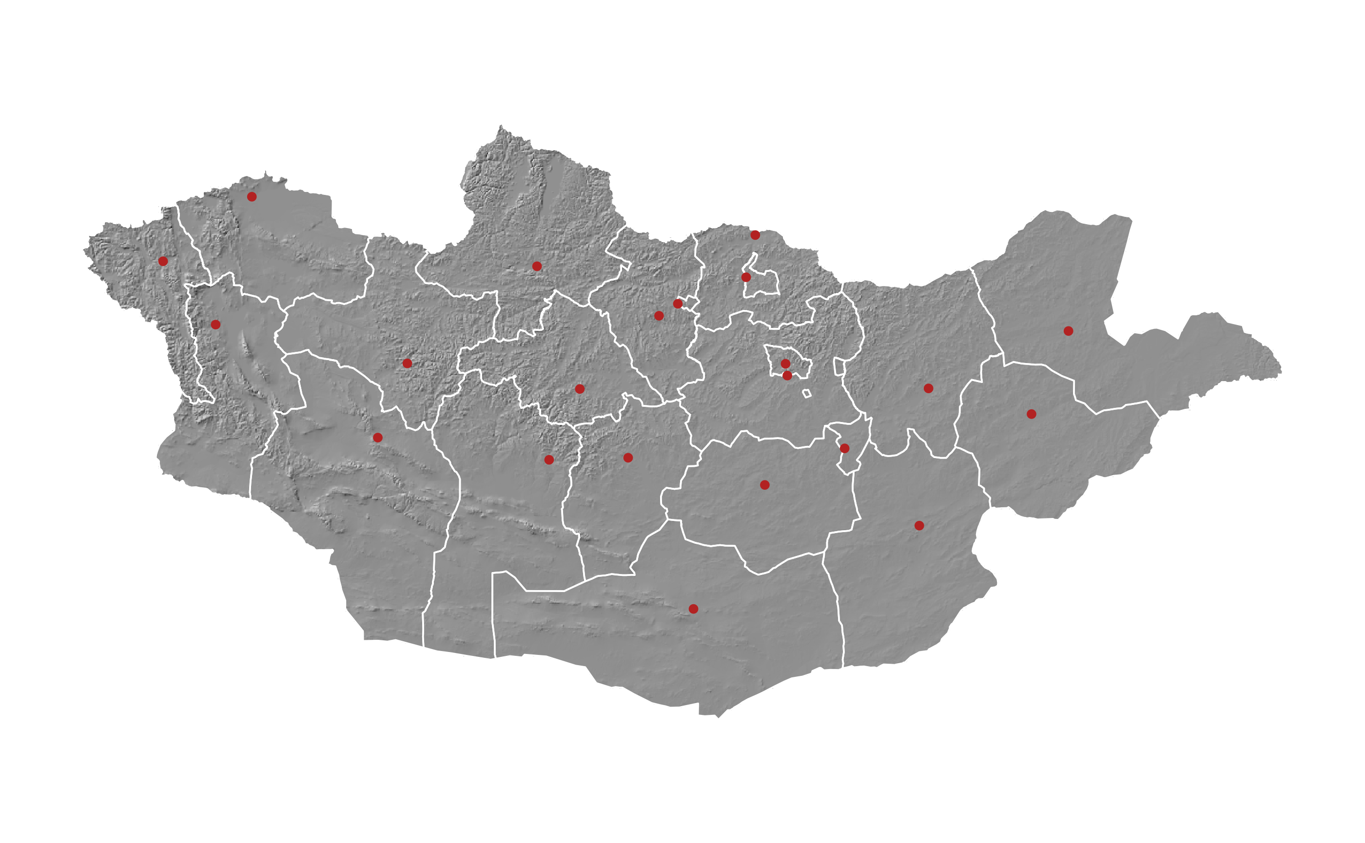
For one area, 90 m detail:
mn_map(mn_hillshade("90m", within = "Ulaanbaatar"), caption = FALSE) +
  geom_sf(data = mn_ub_districts(), fill = NA, colour = "firebrick")
#> Warning: Raster pixels are placed at uneven horizontal intervals and will be shifted
#> ℹ Consider using `geom_tile()` instead.
#> Raster pixels are placed at uneven horizontal intervals and will be shifted
#> ℹ Consider using `geom_tile()` instead.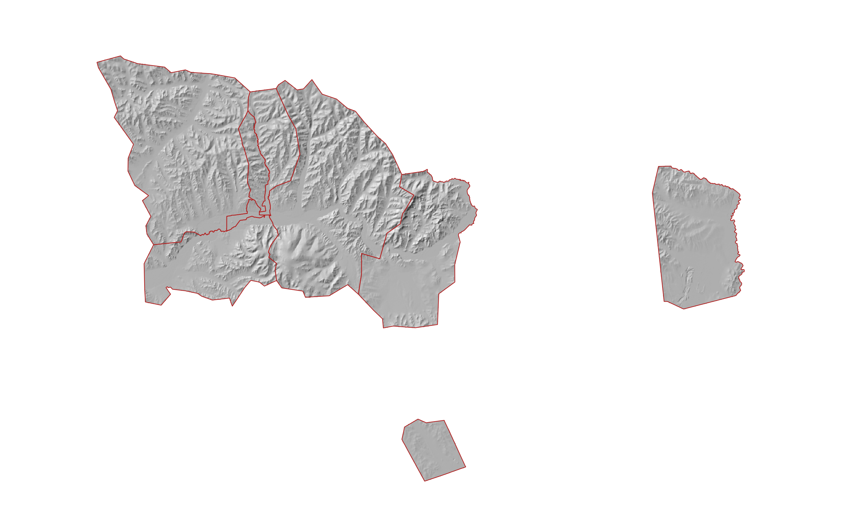
Population
mn_zonal() adds up the grid for any set of polygons, for
example soums:
pop <- mn_population(2025)
soums <- mn_zonal(pop, mn_soums(), name = "population")
mn_map(soums, fill = population / area_km2, trans = "log10",
       title = "People per km2 by soum, 2025 (WorldPop)")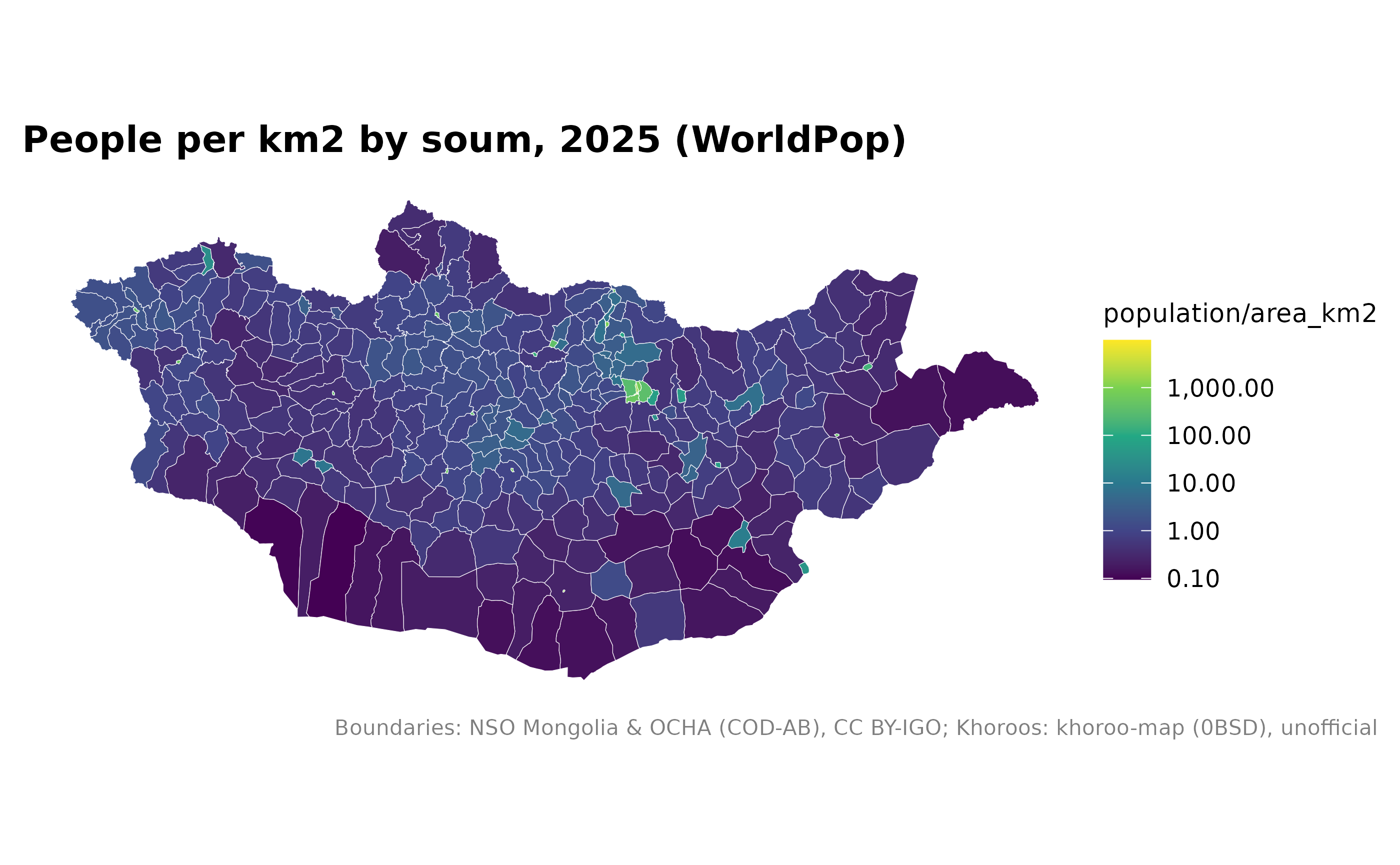
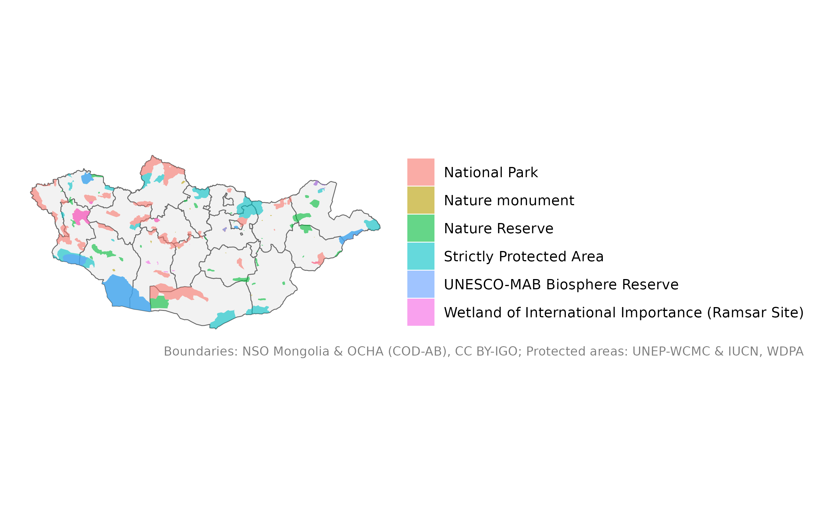
Protected areas
The World Database on Protected Areas may not be redistributed, so it is downloaded from UNEP-WCMC on first use:
pa <- mn_protected_areas()
mn_map(mn_aimags(), caption = FALSE) +
  geom_sf(data = pa, aes(fill = desig_eng), alpha = 0.6, colour = NA) +
  labs(fill = NULL, caption = mn_citation(c("admin", "wdpa")))